I plan to write a series documenting how to progressively tune a GEMM kernel from a basic version to the optimal performance on B200 (1840 TFLOPS). The related code is open-sourced at GitHub - deciding/cutex. You can run it directly using Modal — just install Modal and you’re ready to go, no B200 required.
Currently, most available CuTe examples are either highly refined industrial implementations or relatively basic demos. There’s a lack of systematic demonstrations of tuning strategies and intermediate versions. This series aims to fill this gap.
TL;DR: Summary
- Current Progress: This article implements a “small but complete” basic version (performance ~340 TFLOPS, final version is 1840 TFLOPS). The initial focus isn’t on ultimate performance, but on establishing a clear programming model.
- Core Problem: CuTe DSL’s extreme flexibility easily leads to “shape dizziness” and hard-to-debug potential bugs.
- Optimization Strategy: By actively giving up some flexibility and establishing strict naming conventions and shape tiling paradigms, we can significantly reduce error rates and maintain high code readability even after multiple layers of partitioning.
- Key Conclusions:
- Naming Convention ([Level][Operation/Result][DataSource]): For example, tCgA represents the Tile sliced from Global Memory A for the current Thread to execute MMA C multiplication.
- Implicit Input/Output Constraints of APIs:
local_tile: Output is flattenedpartition_*: Typically accepts Flat shaped inputtma_partition: Does NOT accept Flat shape; input must be hierarchical (nested) shape (tma_tile, *Rests) after operations likegroup_modes.
- Logical Hierarchy of Shapes: Matrix tiling follows a progressive relationship at physical and logical levels: Block (TMA) > MMA > EPI > Store. Understanding this chain is the foundation for deriving the final Tensor shape.
+-----------------------------------------------------------------------+
|                    CuTeDSL Variable Naming Convention Diagram         |
+-----------------------------------------------------------------------+
|                                                                       |
| Structure: [ Prefix ] [ Core ] [ Suffix ]                             |
| Meaning:   Scope      Operation   Location                            |
|                                                                       |
| Mapping Table:                                                        |
|   t : Thread       A : TMA Load A   gA : Global Mem A                 |
|   b : Block        B : TMA Load B   sA : Shared Mem A                 |
|   C : MMA Op (C)  RS: Reg to SMem  rA : Register A                    |
|   ...                                   tA : TMEM A (B200)            |
|                                          sC : Shared Mem C            |
|                                                                       |
+-----------------------------------------------------------------------+
| Typical Example Analysis 1:                                           |
|                                                                       |
| t C gA                                                                |
| │ │ │                                                                 |
| │ │ └─ [Location] : Global Memory A (gA)                              |
| │ │                                                                   |
| │ └──── [Operation]: Represents the MMA Op (C) requirement            |
| │                                                                     |
| └─────── [Scope] : Current Thread (t) perspective                     |
|                                                                       |
| Semantics: A Tile view partitioned from Global Memory A (gA) to       |
| satisfy the current Thread's MMA Op (C) requirement.                  |
|                                                                       |
+-----------------------------------------------------------------------+
| Typical Example Analysis 2:                                           |
|                                                                       |
| t RS sC                                                               |
| │ │ │                                                                 |
| │ │ └─ [Location] : Target is Shared Memory C (sC)                    |
| │ │                                                                   |
| │ └───── [Operation]: Store action from Reg to SMem (RS)              |
| │                                                                     |
| └──────── [Scope] : Executed by current Thread (t)                    |
|                                                                       |
| Semantics: The current Thread (t) executes a Store operation from     |
| Register to Shared Memory (sC).                                       |
|                                                                       |
+-----------------------------------------------------------------------+
1. Pain Point: Cognitive Burden in CuTe DSL Development
When writing CuTe DSL, a significant pain point is that Tensor sizes are often hard to understand intuitively. Even with print outputs, seeing nested shapes like ((64,1), 1, ((1,4), 1, 1)) brings considerable cognitive burden.
The root cause is too much flexibility. Taking TMA, MMA, or TMEM shape operations as examples, due to the API’s high flexibility, developers can often debug and piece together a correct result (for example, changing the above shape to ((64,1), 1, 1, (1, 4, 1, 1)) also works). But the cost is a sharp decline in code readability.
Additionally, compared to Tile-based DSLs (like Triton, where developers mainly focus on CTA-level tiling), CuTe exposes many SIMT-level memory and synchronization details. For example, under 2SM MMA architecture, how should TMA mbar’s expect_tx be dynamically adjusted? When to judge is_leading_cta? How to allocate Consumer thread numbers? These details easily cause errors.
Therefore, writing CuTe is extremely challenging work. There are many guides introducing CuTe syntax, but without specific operator context, it’s hard to develop deep understanding.
This series is named 【Anti-Dizzy】 series, with the core purpose: When writing code initially, clearly define Tensor shapes, API expected inputs, and the collaboration pattern between Producer and Consumer. This allows us to focus on performance tuning rather than meaningless debugging.
2. Convention 1: Establish Structured Naming Paradigm
My first suggestion: Actively limit some degrees of freedom of CuTe DSL and form a fixed naming and Shape style.
Here’s my coding convention (this convention is consistent with some excellent official examples):
When we see tCgA or tAgA, what do they respectively represent?
- Suffix (Data Source & Memory Level):
gArepresents Matrix A in Global Memory,sArepresents Shared Memory,rArepresents Register. On Blackwell architecture,tArepresents TMEM. - Prefix (Thread Level):
trepresents Thread level,brepresents Block (CTA) level. - Middle Letter (Operation Attribute): In
tAsA, the firstAdoesn’t refer to “Matrix A”, but represents an Op (Operation). This carries the spirit of compiler IR: an identifier represents both the Value and the Op that generates it. Here,Arepresents thetma_load Aoperation. Similarly, intCgA,Crepresents the MMA multiplication operationC = A x B.
Comprehensive Analysis:
The meaning of tCgA: To satisfy the current Thread’s MMA multiplication operation (C) needs, the Tile view sliced from Global Memory A (gA).
(Note: This doesn’t mean GEMM directly reads A from Global Memory for computation. Instead, it represents that tCgA describes the data layout required for MMA. Subsequently, this requirement is passed to tma_partition to generate tAgA for actual TMA load operation.)
Naming Principles for Other Operations:
For operations like tma_store, tmem_load, smem_store, it’s recommended to give up the “naming by result” approach and instead directly describe data flow. For example, use tRSsC to represent the Store operation from Register (R) to SMem (S). The part of sC needed by this thread is tRSsC.
For Block-level tiling, although TMA logically manages the entire Block and strictly should use b prefix, given the community already has extensive usage of tAsA, to reduce reading cost, it’s recommended to uniformly use t as prefix.
For original Tensors not involving partition:
mC: Represents the entire matrixgC: Represents the Global Memory slice responsible for current CTAsC: Represents the pointer in Shared Memory
3. Convention 2: Clarify Input/Output Constraints of Shape Transformation APIs
Unlike Triton’s macro-level operations like splat and split, CuTe requires fine-grained control at Thread and Op dimensions. Here are three most fundamental Divide operations:
tiled_divide:((TileM, TileN), RestM, RestN, L, ...)zipped_divide:((TileM, TileN), (RestM, RestN, L, ...))flat_divide:(TileM, TileN, RestM, RestN, L, ...)
These three are easy to understand literally, but the key lies in their implicit constraints in actual APIs.
Note that for logical_divide, although it is different from tiled_divide in the cpp documents, it behaves the same as it in cutedsl
I. local_tile: Slice with Coordinates + Unfold
local_tile internally calls zipped_divide, then obtains Rest part data based on coord, and finally unfolds the Tile part. Therefore, the return value of local_tile is always a Flat format Tensor.
Example Derivation:
(1024, 256), tiler: (128, 64), coord: (0, None) evolution:
zipped_divide(128, 64), (8, 4) → indexing(128, 64), 4 → unfold 128, 64, 4
Two common usage patterns:
- Pass specific coord: Advantage is being able to use
projparameter to precisely locate current CTA’s Tile. - Pass
(None, None, ...)as coord: Advantage is when writing Persistent Kernel, you can pre-define gA’s layout and dynamically get Tile inside loop based on dynamic coord.
II. thr_op.partition_*: Thread-Level Fine-Grained Partitioning
Core Ops in Cutlass are mainly Copy and MMA (including many subclasses like Ld16x64bOp, MmaF16BF16Op). Standard construction flow: op_atom → tiled_op → thr_op.
Example:
tmem_atom = cute.make_copy_atom(
    tcgen05.Ld32x32bOp(tcgen05.Repetition.x64),
    cutlass.Float32,
)
This corresponds to ptx tcgen05.ld.sync.aligned.32x32b.x64.b32
tmem_tiled_copy = tcgen05.make_tmem_copy(tmem_atom, tensor)
This creates a CopyOp specially adapted for tensor based on layout information provided by tensor.
Finally:
tmem_thr_copy = tmem_tiled_copy.get_slice(tidx)
Gets current thread’s CopyOp. We can use it to slice tile under current thread:
tTRtC = tmem_thr_copy.partition_S(tCtAcc_epi)
Core Constraint: Assuming the shape passed to partition_* is flattened (M, N, L), its output must be: (atom_tile, RestM, RestN, L). This atom_tile varies by op: MMA might be (Atom_MMA_M, Atom_MMA_K), e.g., (128, 16), while tmem load might be ((Atom_TMEM_V, Atom_TMEM_T), Rest_TMEM_V), e.g., ((64, 32), 1). But ignoring details, at the abstract level, it’s a very clear result. The difference from local_tile is that its atom_tile is not unfolded.
III. tma_partition: API with Strict Input Format
A common misconception is treating tma_partition and partition_* as equivalent. Actually, their input requirements are fundamentally different.
Input Constraint: tma_partition typically doesn’t accept Flat shape input; it needs a hierarchical form processed by tiled_divide or group_modes, i.e., (tma_tile, RestM, RestN, L). This explains why in code, you often need to first use cute.group_modes to pack local_tile’s Flat result before feeding it to tma_partition.
Output: Its output structure is still (tma_tile, RestM, RestN, L), except the internal tma_tile is converted to format meeting TMA hardware requirements. The nested hierarchy level doesn’t change.
Example: If local_tile’s result is (128, 64, 16) → (bM, bN, RestK), we first group_modes to ((128, 64), 16) → ((bM, bN), RestK) → (tma_tile, RestK), then tma_partition(((64, 128), 1), 16) → (tma_atom_tile, RestK). If we understand (128, 64) as tma_tile, then ((64, 128), 1) is just tma_tile conforming to tma atom tile format. Actually, the shape hasn’t changed before and after.
Note that, many codes use tCgA instead of gA (the local_tile result) as the input to tma_partition.
In this case, ((128, 16), 1, 4, 16) if first group_modes to (((128, 64), 1, 4), 16) -> ((mma_atom, *mma_rests), RestK)
Actually, (mma_atom, *mma_rests) can still be treated as tma_tile. And both inputs give you the same partitioned results.
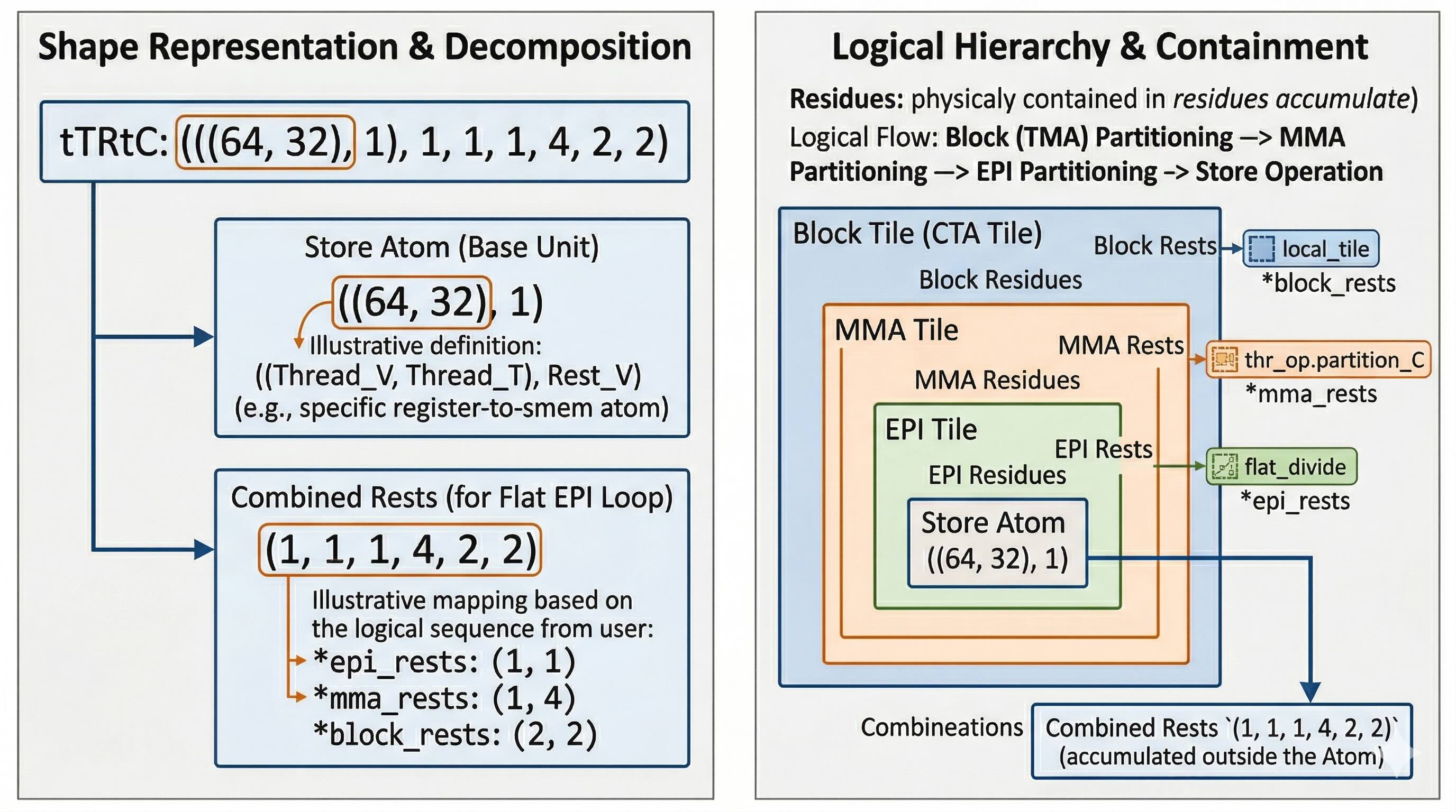
4. Ultimate Verification: Parsing Multi-Layer Partitioned Shape Hierarchy
After a series of complex API calls, how to ensure the final Shape meets expectations? This requires establishing a clear logical hierarchy structure:
Block (TMA) > MMA > EPI > Store
- Block/TMA Level: Each Block handles a larger Tile, TMA executes CTA-level Load operations.
- MMA Level: Block Tile is further divided into multiple MMA blocks (e.g., if K dimension ceiling is 16 and BLOCK_K is 64, need to execute 4 MMA operations).
- Epilogue (EPI) Level: To alleviate register pressure, MMA results are usually artificially flat_divided into multiple batches for Epilogue operations.
- Store Level: Finally, when writing data back, need to further divide based on specific Store Op’s hardware instruction limits.
Mapped to final Tensor shape, it presents a strict nested form from inside to outside:
*(st_atom, *epi_rests, *mma_rests, *block_rests)
Typical Chain Derivation
Example 1: Matrix A Data Flow (Let M, N, K = 1024, 1024, 1024, bM, bN, bK = 128, 256, 64)
gA(No partition):(128, 64, 16)→ corresponds to(*block)tAgA(After TMA partition):(((64, 128), 1), 16)→ corresponds to(tma_atom ((64, 128), 1), *block_rests)tAsA(SMem perspective):((8192, 1), 3)→ corresponds to(tma_atom (8191,1), *buffer)(Note: SMem space is limited, usually uses Software Pipeline buffer size instead of block reduction size)tCgA(MMA perspective read requirement):((128, 16), 1, 4, 16)→ corresponds to(mma_atom (128, 16), *tma_rests (1, 4), *block_rests (16))tCrA(Register stored SMem descriptor):(1, 1, 4, 3)→ corresponds to(mma_atom (1), *tma_rests (1, 4), *buffer (3))
Note that “no partition” means this step hasn’t undergone partition operation, and next it needs to be passed to a partition operation, so the shape will be fully expanded.
Note: Although tCrA is a register, it actually stores SMem descriptor, so the entire mma_atom will be 1.
Example 2: Matrix C Epilogue & Write-back (Let bM, bN, bK = 256, 512)
gC(No partition):(256, 512)→(*block)tCgC(MMA perspective on C):((128, 256), 2, 2)→(mma_atom (128, 256), *block_rests)tEPIgC(EPI partition perspective):(128, 64, 1, 4, 2, 2)→(*epi_tiler (128, 64), *mma_rests (1, 4), *block_rests)tTRtC(Before Store operation):(((64, 32), 1), 1, 1, 1, 4, 2, 2)→(st_atom ((64, 32), 1), *epi_rests (1, 1), *mma_rests (1, 4), *block_rests)tTRrC(Register write-back view):((64,1),1,1)→(st_atom (64, 1), *epi_rests)
(Note: In tTRrS stage, to reuse registers in loops, we usually merge *epi_rests, *mma_rests, *block_rests into one flattened loop body (Flat Loop), so the register view shape no longer contains these outer dimensions.)
(Note2: (64,32) represents a warp, so from 128 to 32 — actually the shape hasn’t changed.)
Conclusion
By incorporating shapes and variable names into this rigorous convention system, we can largely eliminate blindness in underlying development. When reading variable names or checking their Shapes, you can quickly map which hardware operation level they belong to.
Mastering this “anti-dizzy” model, when we subsequently introduce advanced optimization strategies like Software Pipelining and TMA Multicast, we can ensure the logic remains clear and controllable. In the next article, based on this foundation, we will officially begin the tuning process towards 1840 TFLOPS performance.